
Machine Learning in Dental Radiology
- Michelle Howe

- Jan 1, 2020
- 8 min read
Updated: May 29, 2020
Study Summary: A machine learning model was created and trained using convolutional neural networks for object detection in dental radiographs. The model was evaluated based on its accuracy of labeling teeth, periapical pathology, and direct and indirect restorative materials on periapical and bitewing radiographs.
Other contributor: Albert Shim

Introduction:
Machine learning, or predictive analytics, is a subset of artificial intelligence based on the idea that computer systems can learn from data, identify patterns, and make predictions without being explicitly programmed. Advances in machine learning facilitated the creation of many complex technologies of this generation. It is the cornerstone of Photo Tagging applications like Facebook face detection, predictive text, GPS traffic and route time prediction, and automatic sorting of email spam. In recent years, machine learning has been applied to the medical field and has successfully been used to detect abnormality in lower extremity radiographs, diagnose pneumonia in chest radiographs, and classify skin cancer using images of the integument. Medical applications of machine learning have become so promising that in 2018, Stanford’s Center for artificial intelligence in medicine and imaging was founded.
Compared to the medical field, the dental field appears to have limited applications of machine learning to date. Our aim was to use transfer learning to create a model that will be able to detect and label teeth, periapical pathology, and restorative materials with practical and clinically relevant accuracy.
Methods
Dataset Preparation
The overall dataset consists of intraoral radiographs which were collected from the University of Utah School of Dentistry. The images were anonymized by Romexis Imaging software before being exported to encrypted hard drives (as an added precaution). Initially, 4000 images were harvested for processing, however, most of them were deemed unnecessary since the Mask RCNN model was able to produce decent results with just a few hundred annotated images.
Labelbox was used to annotate all instances of each of the following categories:
(1) tooth, (2) periapical pathology, (3) mental foramen, (4) calculus, (5) composite, (6) amalgam, (7) PFM crown, (8) ceramic crown, (9) bridge, (10) implant, (11) root canal therapy, (12) post, (13) root tip, (14) caries
To make the training go as smoothly as possible, only the “Tooth” category and the associated images were included in the initial training sessions. Each object instance in a radiographic image was drawn using a polygon tool and assigned a category in the aforementioned list. The annotations were exported in Labelbox’s new format, which turned out to be incompatible with Microsoft’s COCO format (A widely used format in ML). Custom code had to be written in the Python programming language to reformat the LabelBox annotations into a usable COCO format.
Once the annotations file was properly formatted into COCO, the annotations were randomly divided into two JSON (JavaScript Object Notation) files as “instances_train” and “instances_val”. The two JSON files were used as a template for dividing the dataset images into two separate folders with a ratio of 80:20 (train:val). The separated annotations with their respective images were inspected visually using the provided Jupyter notebook called “inspect_data.ipynb” in the Github repository for the latest commit of Mask R-CNN (https://github.com/matterport/Mask_RCNN). Once the labels were visually inspected to make sure the reformatting process did not mix up the annotations, training on the Mask R-CNN architecture was started for 100 epochs for the heads layer, 150 epochs on ResNet 4+ layers and up, and 300 epochs for all layers.
Model Architecture
The Mask R-CNN architecture was used to train a simple tooth detection model. Mask R-CNN is merely an extension of the Faster R-CNN architecture and only adds a branch for predicting segmentation masks on each Region of Interest (RoI) produced by the Faster R-CNN, in parallel with the existing branch for classification and bounding box regression. The mask branch is a small Fully Connected Convolutional Network applied to each RoI, predicting a segmentation mask for each pixel in an image. Due to Mask R-CNN’s simplicity in design, computational overhead is reduced and easy to implement quick model prototyping.
ResNet101 was used for the backbone architecture with pre-trained weights from imagenet to perform transfer learning instead of using randomized initial weight values to save on time. Before the images are fed into the model for training, they are resized to a square shape with original aspect ratios kept using zero padding so that a batch size of 2 images could be used for every step. Since the radiographs are in a grayscale format (meaning one channel instead of three for RGB color) and the architecture takes in three channels, the values from the grayscale channel were duplicated into the other two channels for RGB.
A learning rate of 0.001 with a momentum of 0.9 and a weight decay of 0.0001 was found to be optimal for consistent training and validation loss decrease. Gradient clipping normalization of 5.0 was used to prevent the gradient from exploding as stochastic gradient descent takes place during training.
This model was then used to train, validate, and test the model groups in this study.
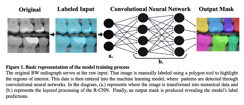
The graphics above show what the machine learning model sees as it tries to find features in a dental radiograph (189 layers)
Results
Tooth Model
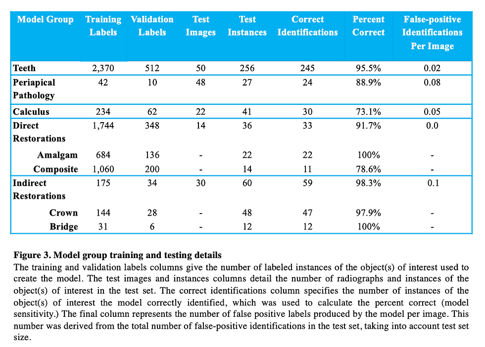
A model has successfully been developed that identifies teeth in BW and PA radiographs. Data supports that this model is accurately detecting teeth. The model was trained on 463 training images and 100 validation images. The test set consisted of 50 images containing 256 teeth. 245 teeth were correctly identified, while 11 were not identified as teeth by the model. Therefore, our model demonstrated 95.5 % sensitivity for this category and 0.02 false-positive identifications per image. Of the 11 teeth that the model failed to identify as teeth, 5 were canines.

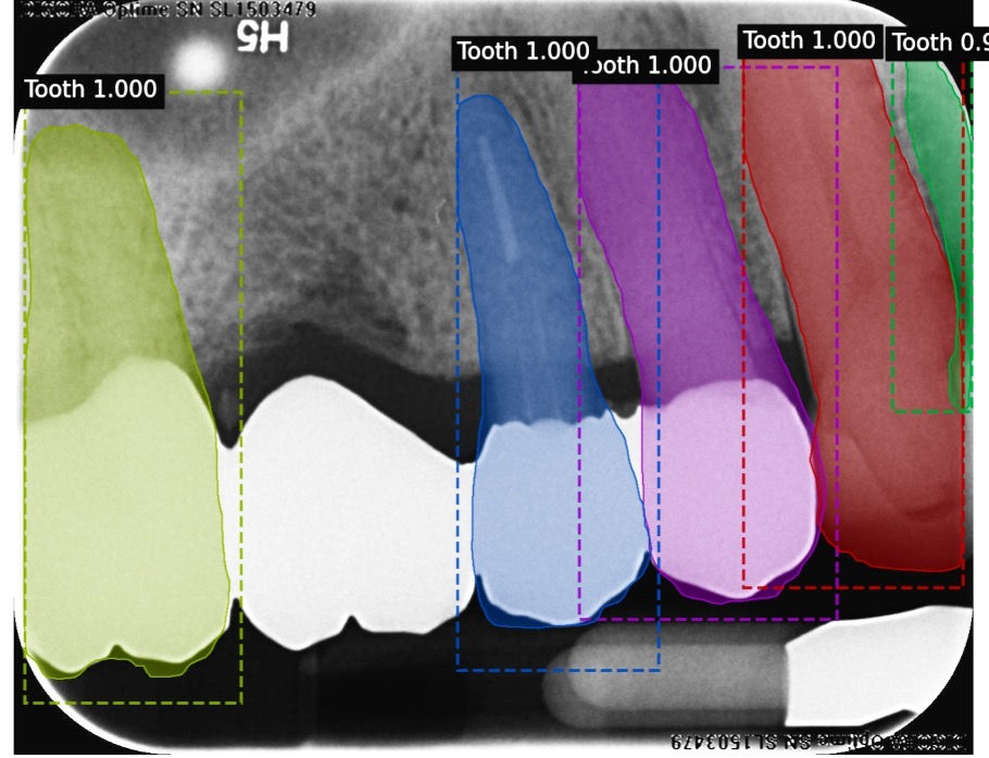
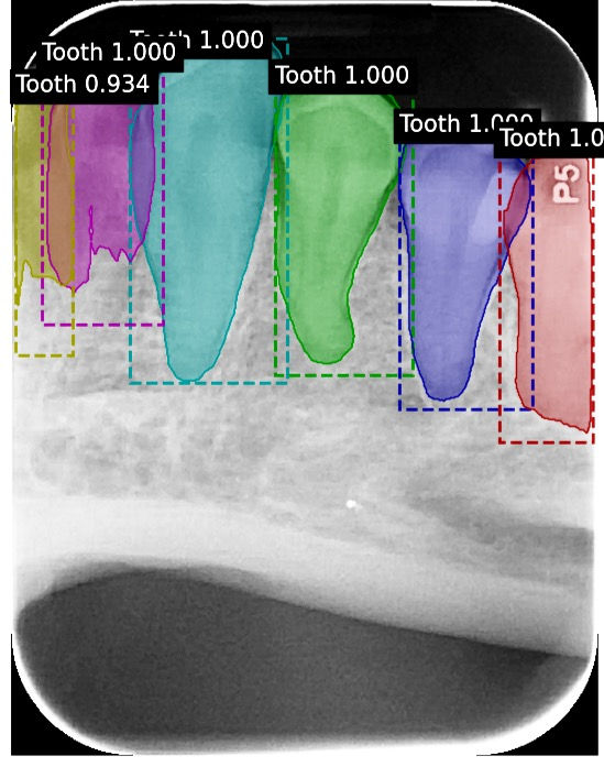
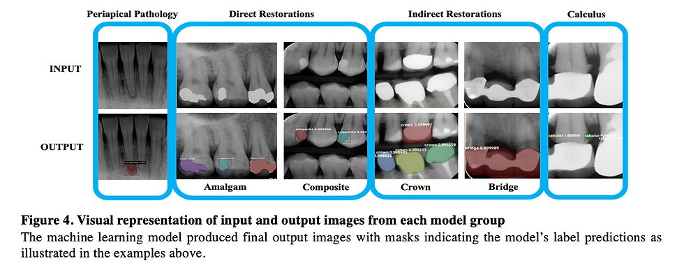
These are examples of labeled images that were produced by our machine learning model. The computer managed to produce accurate tooth masks for all teeth that were present in these BW and PA radiographs.
This image produced by our tooth model demonstrates that our trained model can produce accurate results even in the presence of extreme distortion and overlap.
Periapical Pathology Model
The model was trained with 52 PA radiographs containing labels for periapical pathology. 20% of these labels were used for the validation dataset. In the test set were 27 total radiographically visible instances of periapical pathology. Our model accurately identified 24 of the 27 abnormalities. Therefore, our model demonstrates 88.9% sensitivity regarding periapical pathology identification and 0.08 false-positive identifications per image. Our model failed to identify 3 instances of PA pathology. We would expect higher accuracy with more radiographs of periapical pathology for training and validation. Due to a very small sample size of only 52 radiographs containing periapical pathology, there were some anticipated false-positive labels. We anticipated that the maxillary sinus and mental foramen would be mistakenly identified as periapical pathology due to the similarities in shape and radiograph contrast and because we did not train the model to recognize these anatomical structures. To our surprise only one false positive identified a mental foramen as periapical pathology and no maxillary sinus was identified as periapical pathology even though there were several instances of each of these in the test set. 3 other false positives were identified on the test set where no periapical pathology is noted. Since we have limited radiographs of this category this result was expected and results obtained are promising for computer periapical pathology object detection.
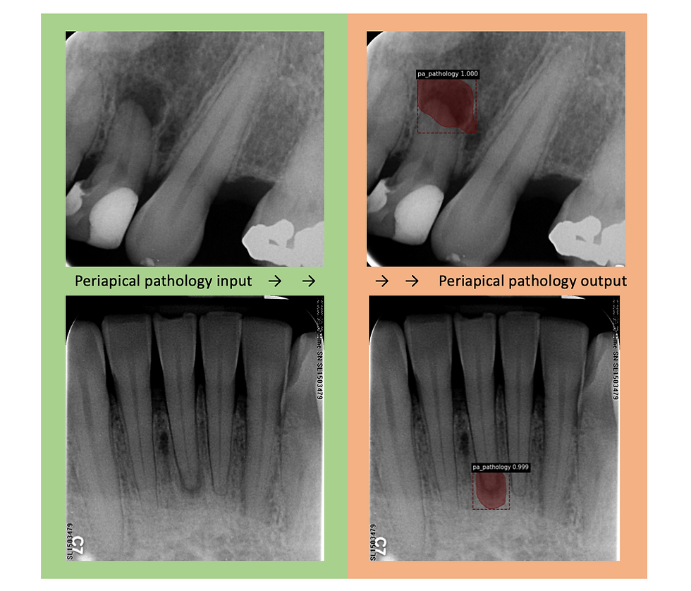
Figure 3: Two examples of object identification that the periapical pathology model produced. Both show that the model accurately produced masks over the true pathology in the output radiograph.
Direct Restoration Model: Composite and Amalgam
The model was trained using 167 PA and BW radiographs with 33 radiographs being used for the validation dataset. In total there were 1,744 composite and amalgam restoration labels combined within the 167 radiographs. There were 684 amalgam restoration labels and 1,060 composite restoration labels used for training and validation. In the test set, 14 PA and BW radiographs were used with a total of 36 composite or amalgam restorations contained within. Of the 36 total direct restorations present, our model accurately identified 33 correctly. Therefore, our direct restoration model possesses 91.67% sensitivity for identifying composite and amalgam restorations with 0.00 false-positive identifications per image. There were 22 amalgam restorations in the test set and all 22 were correctly identified as amalgam, so our model has the capability to identify amalgam restorations with incredible accuracy. Of the 14 composite restorations in the test set, 3 failed to be identified, so our model only correctly identified 11 of the 14 composite restorations. The most promising result, however, is that our model never incorrectly labeled an amalgam restoration as a composite restoration and vice versa demonstrating that our model is distinguishing these materials from each other as well as distinguishing tooth structure from restorations. Due to the occasionally subtle opacity of some composite restorations compared to the amalgam restorations, we believe we may have obtained more representative results with a bigger composite restoration test dataset.
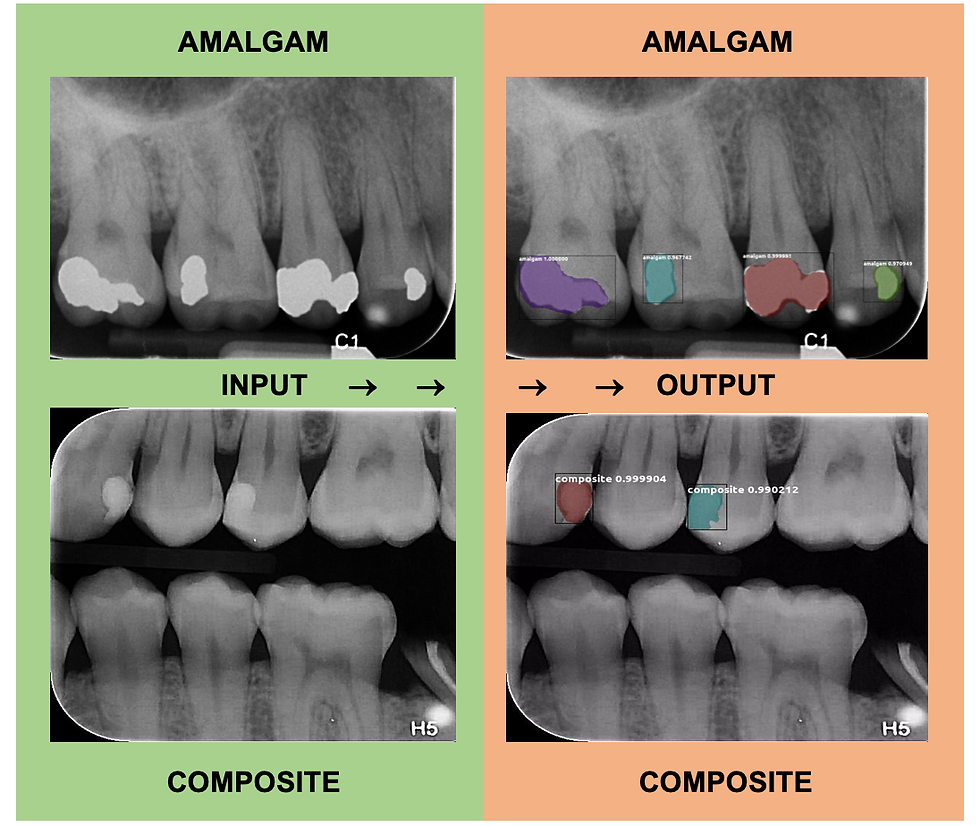
Figure 4: Two examples of object identification that the direct restoration model produced. Both show that the model accurately produced masks over the amalgam and composite restorations.

This output image from the direct restoration model shows only 3 of 4 composite restorations being correctly identified. The composite on #20 was not identified as a restoration by the computer.
Indirect Restoration Model: Crowns and Bridges
For the purpose of this study the "crown" labels included instances of both ceramic and PFM crowns. The model was trained using 137 PA and BW radiographs with 34 radiographs being used for the validation dataset. In total there were 144 crown labels and 31 bridge labels in the training dataset. The test set consisted of 30 PA and BW radiographs containing crowns, bridges, or both. There were a total of 48 crowns and 12 bridges in the test set. Overall, the indirect restoration model demonstrated 98.3% sensitivity with 0.1 false-positive identifications per image. The model demonstrated 97.92% sensitivity for detecting crowns as 47 out of the 48 crowns were correctly identified, while demonstrating 100% sensitivity at detecting crowns as all 12 bridges were correctly identified. The test set model output showed that there were 3 false positive crown labels produced, however, as natural tooth structure was mislabeled as a crown. Out of 72 natural teeth present in the 30 test radiographs, a false positive label was only produced 4.12% of the time. Similarly, one false positive bridge label occurred, where natural teeth were mistaken for a bridge. Because of the demonstrated success of this model, we plan to separate the crown labels into ceramic crown vs PFM crown categories in the future.
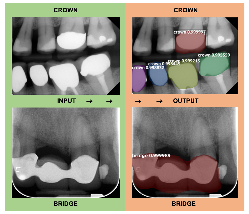
Figure 5: Two examples of object identification that the indirect restoration model produced. Both show that the model accurately produced masks over the crowns and bridges present in the BW and PA radiographs.

This output image from the indirect restoration model shows that the model was accurately able to identify crowns and bridges and distinguish them from each other even when present in the same radiograph.
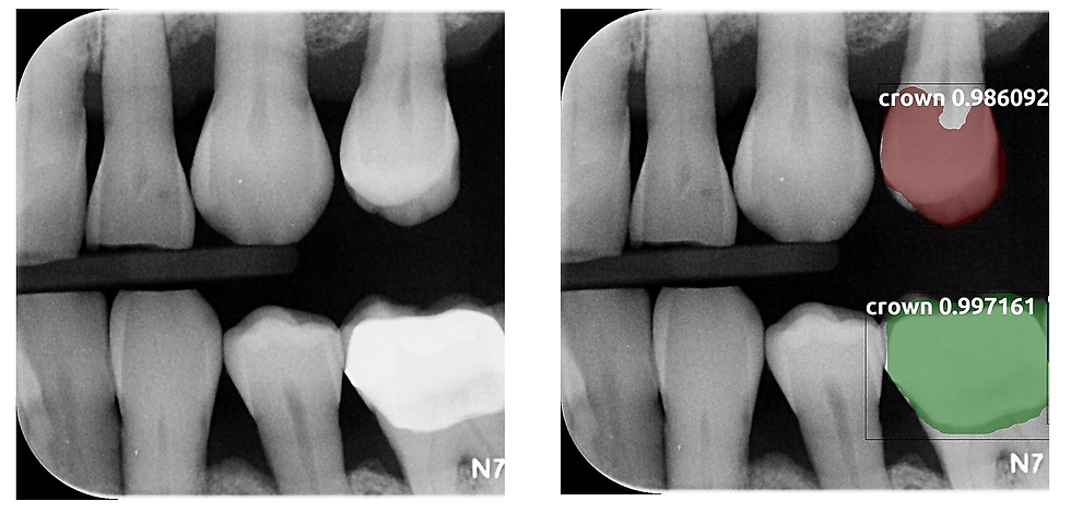
This input and output image shows that natural tooth #12 was mistakenly labeled as a crown, representing a false positive label. In contrast, tooth #19 was correctly given a crown label.
Calculus Model
The model was trained using 80 PA and BW radiographs with 20 radiographs used for the validation dataset. In total there were 234 calculus labels in the training dataset and 62 calculus labels in the validation dataset. The test set contained 22 PA and BW radiographs with a total of 41 radiographically visible calculus deposits. The model correctly identified 30 of the 41 calculus deposits. Therefore, the model demonstrated 73.17% sensitivity with 0.05 false-positive identifications per image. The model failed to identify 11 calculus deposits, most of which were found on mandibular anterior PA radiographs. The small number of training radiographs coupled with the subtlety and small size of many calculus deposits might explain the lower accuracy found with this model. Only one false positive calculus label resulted, however.

Figure 6: Two examples of object identification that the calculus model produced. Both show that the model accurately produced masks over the calculus deposits present in the radiographs.
Summary of results:

Our model is currently being trained to detect interproximal caries, identify the tooth number, automatically predict root canal working length and calculate horizontal bone loss in PA and BW radiographs. Preliminary results will be posted here when available.
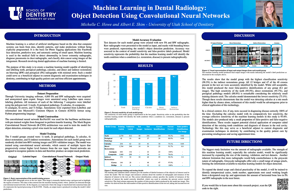
My original project poster can be viewed below.

Comments